North Central and Wabash Headwaters water studies’ boundaries
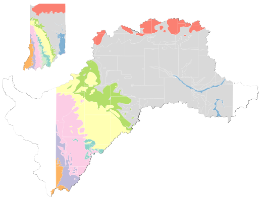
Indiana bedrock
aquifer systems
Significant
groundwater withdrawal facilities
High capacity well range average
Domestic well range average
Principal aquifer composition
Principal aquifer composition
Water study
Blue River, Sanders Groups
Gallons per minute
Gallons per minute
Carbonate-rock
Glacial sand and gravel
Borden Group
North Central Indiana
Subbasin boundaries
Gallons per
minute capacity
Sandstone and carbonate-rock
Buffalo Wallow, Stephensport, West Baden Groups
Surface water sources
Type of use
Wabash Headwaters
Carbondale Group
Major waterways
200
0
10
20
30
40
50
Energy production
500
1,000
1,500
Coldwater, Ellsworth, Antrim Shales
Minor waterways
500
Industry
Maquoketa Group
800
McLeansboro Group
Irrigation
1,667
New Albany Shale
13,500
Miscellaneous
Raccoon Creek Group
Public supply
Silurian and Devonian Carbonates
Trenton, Lexington, and Black River Carbonates
Rural use
North Central and Wabash Headwaters water studies’ boundaries
Indiana
bedrock aquifer systems
Significant ground-
water withdrawal facilities
High capacity well range average
Domestic well range average
Water study
Principal aquifer composition
Principal aquifer composition
Blue River, Sanders Groups
Gallons per minute
Gallons per minute
North Central Indiana
Subbasin boundaries
Glacial sand and gravel
Carbonate-rock
Borden Group
Gallons per
minute capacity
Wabash Headwaters
Type of use
Buffalo Wallow, Stephensport, West Baden Groups
Sandstone and carbonate-rock
Surface water sources
Carbondale Group
500
1K
1.5K
0
10
20
30
40
50
Energy
200
Major waterways
Coldwater, Ellsworth, Antrim Shales
500
Industry
Maquoketa Group
Minor waterways
800
Irrigation
McLeansboro Group
1,667
New Albany Shale
Miscellaneous
13,500
Raccoon Creek Group
Public supply
Silurian and Devonian Carbonates
Rural use
Trenton, Lexington, and Black River Carbonates
North Central and Wabash Headwaters water studies’ boundaries
Indiana
bedrock aquifer systems
Water study
Principal aquifer composition
Significant groundwater
withdrawal facilities
Subbasin boundaries
North Central Indiana
High capacity well range average
Domestic well range average
Blue River, Sanders Groups
Principal aquifer composition
Glacial sand and gravel
Wabash Headwaters
Gallons per minute
Gallons per minute
Borden Group
Gallons per
minute capacity
Carbonate-rock
Buffalo Wallow, Stephensport, West
Baden Groups
Surface water sources
Type of use
Sandstone and carbonate-rock
Major waterways
500
1K
1.5K
0
10
20
30
40
50
Energy
200
Carbondale Group
500
Minor waterways
Industry
Coldwater, Ellsworth, Antrim Shales
800
Irrigation
1,667
Maquoketa Group
Miscellaneous
13,500
McLeansboro Group
Public supply
New Albany Shale
Rural use
Raccoon Creek Group
Silurian and Devonian Carbonates
Trenton, Lexington, and Black River
Carbonates
Excess water
availability
Upstream
subbasins
Upstream
subbasin
Cumulative
excess
water
availability
Excess water
availability
Instream flow
requirement
Subbasin
Excess water
availability
Upstream
subbasins
Upstream
subbasin
Cumulative
excess
water
availability
Excess water
availability
Instream flow
requirement
Subbasin
Excess water
availability
Upstream
subbasins
Upstream
subbasin
Cumulative
excess
water
availability
Excess water
availability
Instream flow
requirement
Subbasin
Excess water
availability
Upstream
subbasins
Upstream
subbasin
Cumulative
excess
water
availability
Excess water
availability
Instream flow
requirement
Subbasin
Wabash Headwaters
subbasin 10
Water study
North Central Indiana
Wabash Headwaters
North Central Indiana
subbasin 16
Wabash Headwaters
subbasin 10
Water study
North Central Indiana
Wabash Headwaters
North Central Indiana
subbasin 16
Wabash Headwaters
subbasin 10
Water study
North Central Indiana
Wabash Headwaters
North Central Indiana
subbasin 16
Wabash
headwaters
subbasin 10
Water study
North Central Indiana
Wabash Headwaters
North Central Indiana
subbasin 16
Historic and future cumulative excess water availability by season and
subbasin
Future
Historic
Cumulative excess
water availability
Winter
Million gallons daily
(MGD)
12 - 498
498 - 1,454
Spring
1,454 - 2,971
2,971 - 4,356
4,356 - 5,819
5,819 - 7,727
7,727 - 9,964
Summer
Fall
Historic and future cumulative excess water availability by season and
subbasin
Future
Historic
Cumulative excess
water availability
Winter
Million gallons daily
(MGD)
12 - 498
498 - 1,454
Spring
1,454 - 2,971
2,971 - 4,356
4,356 - 5,819
5,819 - 7,727
7,727 - 9,964
Summer
Fall
Historic and future cumulative excess water availability by season and
subbasin
Historic
Future
Cumulative excess
water availability
Million gallons daily
(MGD)
Winter
12 - 498
498 - 1,454
1,454 - 2,971
Spring
2,971 - 4,356
4,356 - 5,819
5,819 - 7,727
7,727 - 9,964
Summer
Fall
Historic and future cumulative excess water availability by season and
subbasin
Historic
Future
Cumulative excess
water availability
Million gallons daily
(MGD)
Winter
12 - 498
498 - 1,454
1,454 - 2,971
Spring
2,971 - 4,356
4,356 - 5,819
5,819 - 7,727
7,727 - 9,964
Summer
Fall
Percent change from historic to future cumulative excess water
availability
Winter
Spring
Percent
change
40%
20
0
Fall
Summer
-20
Percent change from historic to future cumulative excess water
availability
Winter
Spring
Percent
change
40%
20
0
Fall
Summer
-20
Percent change from historic to future cumulative excess water
availability
Winter
Spring
Percent
change
40%
20
0
Fall
Summer
-20
Percent change from historic to future cumulative excess water
availability
Winter
Spring
Percent
change
40%
20
0
Fall
-20
Summer
Future cumulative excess water availability exceedance curve
North Central Indiana Regional Water Study, subbasin 6
Million gallons daily
Winter
Spring
6K
Extremely wet: 6%
Extremely wet: 6%
Negative
availability
4K
Average
conditions: 53%
Average
conditions: 53%
Fall
Summer
2K
Extremely dry:
94%
Extremely dry:
94%
Spring
Fall
Values below 0 indicate negative availability
0
Summer
Winter
10
20
30
40
50
60
70
80
90
100%
Exceedance
Future cumulative excess water availability exceedance curve
North Central Indiana Regional Water Study, subbasin 6
Million gallons daily
Winter
Spring
6K
Extremely wet: 6%
Extremely wet: 6%
Negative
availability
Average
conditions: 53%
4K
Average
conditions: 53%
Fall
Summer
2K
Extremely
dry: 94%
Extremely
dry: 94%
Spring
Fall
Values below 0 indicate negative availability
0
Summer
Winter
10
20
30
40
50
60
70
80
90
100%
Exceedance
Future cumulative excess water availability exceedance curve
North Central Indiana Regional Water Study, subbasin 6
Million gallons daily
Winter
Spring
6K
Extremely wet: 6%
Extremely wet: 6%
Negative
availability
Average
conditions: 53%
4K
Average
conditions: 53%
Fall
Summer
2K
Extremely dry: 94%
Extremely dry: 94%
Spring
Values below 0 indicate negative availability
Fall
0
Summer
Winter
10
20
30
40
50
60
70
80
90
100%
Exceedance
Future cumulative excess water availability exceedance curve
North Central Indiana Regional Water Study, subbasin 6
Million gallons daily
Winter
Spring
6K
Extremely wet: 6%
Extremely wet: 6%
Negative
availability
Average
conditions: 53%
4K
Average
conditions: 53%
Fall
Summer
2K
Extremely dry: 94%
Extremely
dry: 94%
Spring
Fall
Values below 0 indicate negative availability
0
Summer
Winter
10
20
30
40
50
60
70
80
90
100%
Exceedance
Future cumulative excess
water availability by
season, subbasin and
climate condition
1
7
2
Indiana Finance
Authority water study
4
North Central Indiana
Wabash Headwaters
5
8
6
2
3
9
9
10
10
1
5
3
6
4
11
8
7
Downstream
basin flow
13
3
12
Tributaries
4
2
5
Mainstem
Wabash
River
Subbasin cumulative excess water availability
The area of each square represents the subbasin’s
cumulative excess water availability under that climate
condition.
1
6
14
8
7
Winter
Spring
Extremely wet
3
9
10
15
Average
5
Negative water
availability
6
1
4
2
Extremely dry
7
10
126 MGD
583 MGD
16
11
9
8
12
1,651 MGD
Subbasin
number,
study area
Range of cumulative
excess water available
per season.
13
15
14
6
Fall
Summer
16
Future cumulative excess
water availability by
season, subbasin and
climate conditions
1
7
Indiana Finance
Authority water study
2
4
North Central Indiana
Wabash Headwaters
5
8
6
2
3
9
9
10
10
1
5
3
6
4
11
8
7
Downstream
basin flow
13
3
Tributaries
12
4
2
5
Mainstem
Wabash
River
Subbasin cumulative excess water availability
The area of each square represents the subbasin’s cumulative
excess water availability under that climate condition.
1
6
14
8
7
Winter
Spring
3
9
10
Extremely wet
15
Average
5
6
1
4
2
Extremely dry
Negative water
availability
7
10
16
11
9
8
12
Subbasin
number,
study area
15
13
14
6
Fall
Summer
16
Future cumulative excess
water availability by
season, subbasin and
climate conditions
1
7
Indiana Finance
Authority water study
2
4
North Central Indiana
Wabash Headwaters
5
8
6
2
3
9
9
10
10
1
5
3
6
4
11
8
7
Subbasin cumulative excess water
availability
13
12
The area of each square represents the subbasin’s cumulative
excess water availability under that climate condition.
Spring
Winter
14
Extremely wet
Average
15
Extremely dry
Negative water
availability
Subbasin
number,
study area
16
6
Summer
Fall
Future cumulative excess
water availability by
season, subbasin and
climate conditions
1
7
Indiana Finance
Authority water study
2
4
North Central Indiana
Wabash Headwaters
5
8
6
2
3
9
9
10
10
1
5
3
6
4
11
8
7
Subbasin cumulative excess water
availability
13
12
The area of each square represents the subbasin’s cumulative
excess water availability under that climate condition.
Spring
Winter
14
Extremely wet
Average
15
Extremely dry
Negative water
availability
Subbasin
number,
study area
16
6
Summer
Fall
Future cumulative excess water availability by season, subbasin and
climate conditions
7
4
5
8
6
10
2
3
9
1
North Central Indiana regional water study
1
2
Wabash Headwaters regional water study
6
8
6
9
10
7
5
12
3
4
11
8
13
14
Subbasin cumulative excess water availability
15
The area of each square represents the
subbasin’s cumulative excess water
availability under that climate condition.
6
16
Winter
Spring
Extremely wet
Average
Extremely dry
Negative water
availability
Subbasin
number
6
Fall
Summer
By: Ted Schurter August 18, 2026
The Indiana Finance Authority’s two recent regional water studies, the North Central Indiana and Wabash Headwaters, explain the location, origin and
extent of those regions’ water resources.
They detail the historic and current levels of water availability, excess water
availability and cumulative excess water availability for each region, and the
subbasins within, and estimate how those metrics may change based on future conditions.
Understanding these concepts and water availability metrics should make interpreting the statewide
water assessment Indiana Gov. Mike Braun ordered completed by the end of 2026 a little
easier.
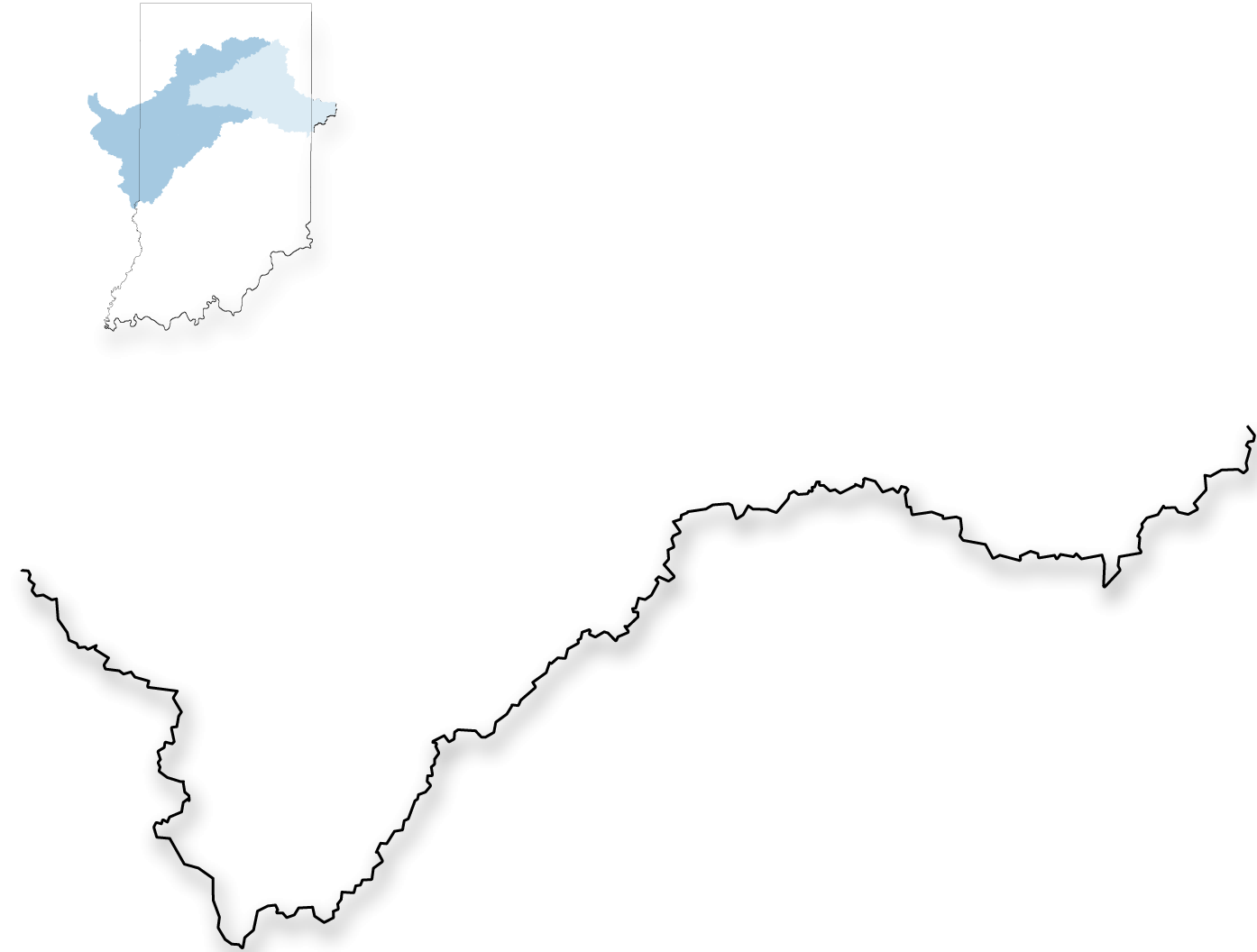
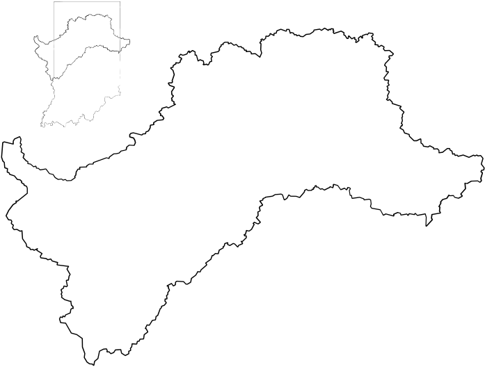
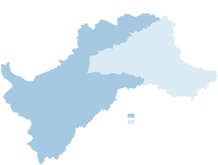
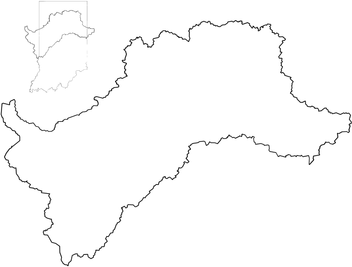
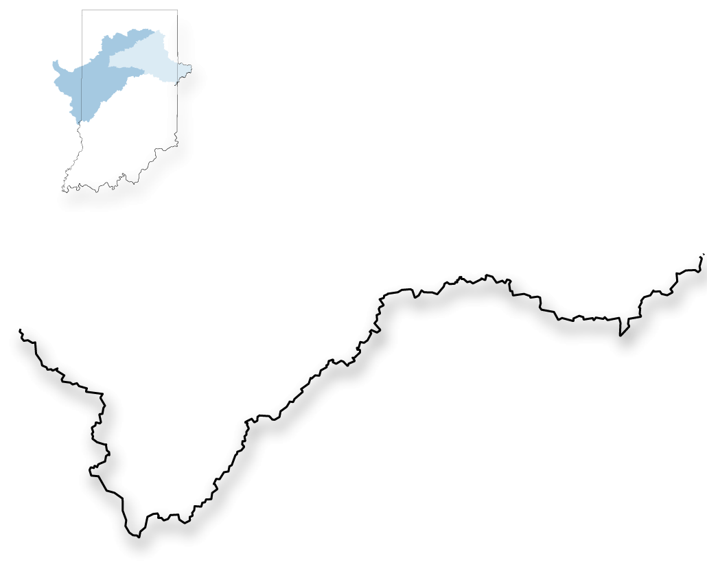
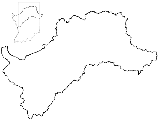
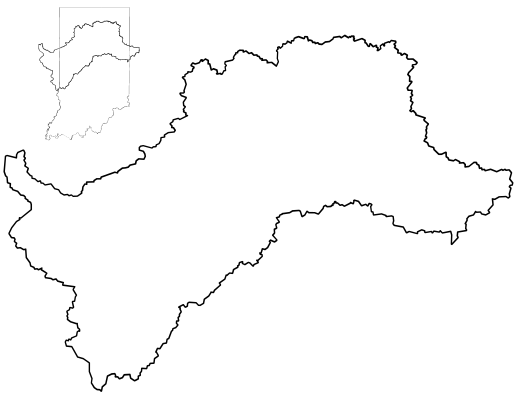
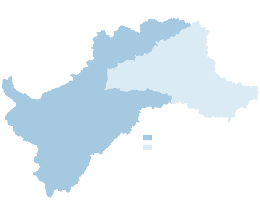
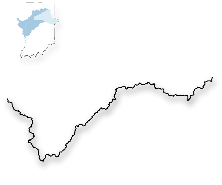
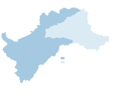
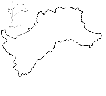
Map showing combined area of North Central Indiana, shaded light blue, and Wabash
Headwaters, shaded darker blue, water studies by the Indiana Finance Authority. A smaller inset
map of Indiana shows their state context.
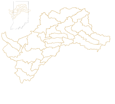
Each study encompasses a region that is divided into subbasins. Their boundaries are delineated
by hydrology, topographic features, and measured streamflow data, not by administrative
boundaries like county or state lines.
Each subbasin drains a specific area, that is the water within it generally flows to a common
point, where the streamflow data is measured.
For each subbasin, water availability is calculated with a formula:
Water availability = Net natural baseflow– net minimum instream flow requirement+subbasin net reservoir release.
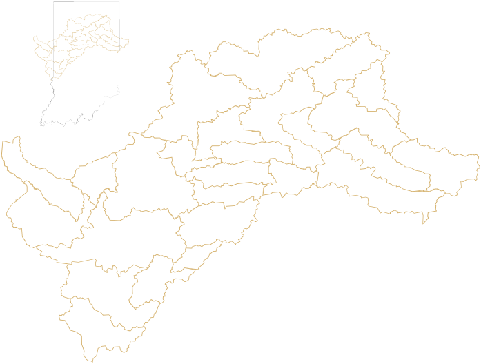
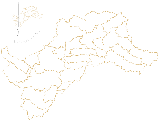
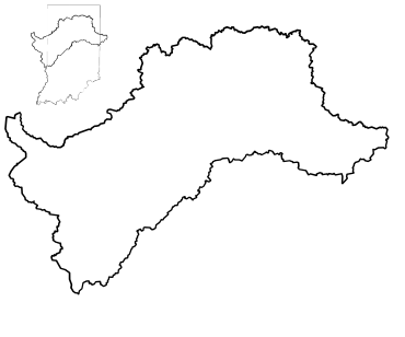
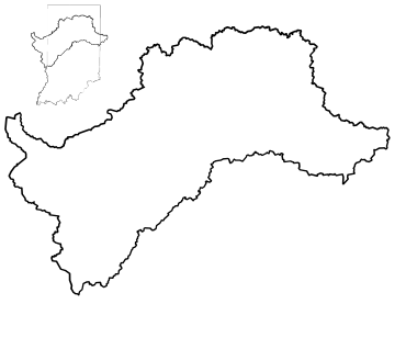
Map showing combined area of North Central Indiana and Wabash Headwaters water
studies by the Indiana Finance Authority and the subbasins within them marked by gold lines. An
inset map in the upper left shows the study areas in the context of the state of Indiana.
Water availability = Net natural baseflow
– net minimum instream flow requirement+subbasin net
reservoir release.
Net natural baseflow is the total groundwater contribution to streamflow within a
subbasin. This is estimated without human influences like water withdrawals or wastewater-return
flows.
The net minimum instream flow requirement is the amount of water that must remain within
a
subbasin to maintain ecosystem health, water quality and recreational use.
Like baseflow and precipitation, the minimum instream flow requirement changes seasonally.
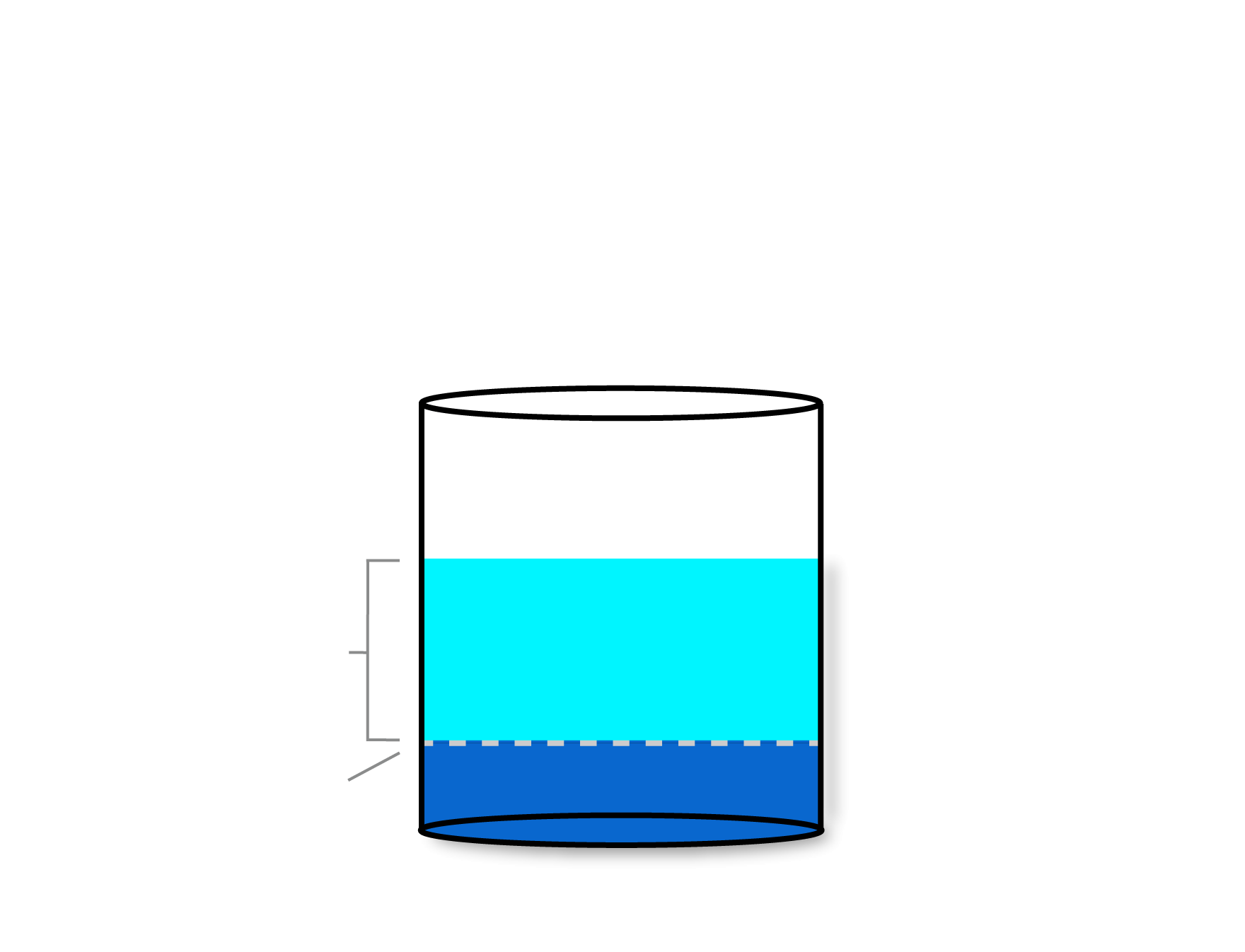
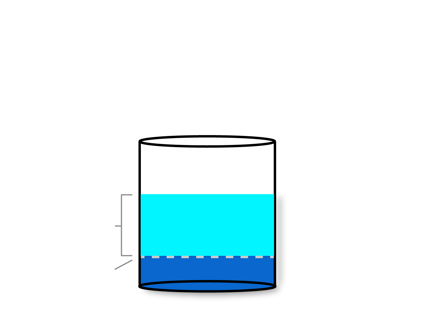
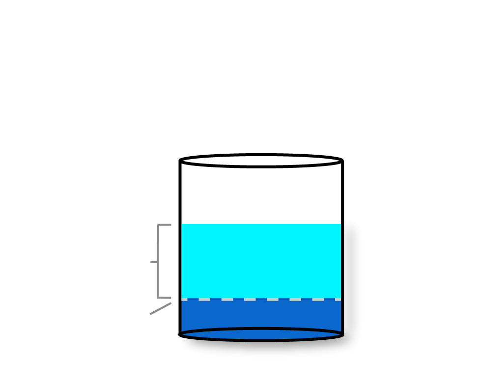
Adjust the slider to see how wet or dry conditions, combined with the
minimum instream flow requirement, affect water availability.
Drier conditionsWetter conditions
Illustration of a cylinder with dark blue water and a fixed dashed gray line at
the bottom labeled 'Instream flow requirement.' An indicator and label show Natural baseflow on
the left and a bracked indicator showing Water availability on the right. Both labels move up
and down when users activate the slider control to show relationship between baseflow, the
instream flow requirement and water availability.
Water availability: baseflow
Natural baseflow originates from aquifers so understanding their relationship to the subbasins
above them is important.
An aquifer is any collection of geologic material that is saturated with enough water to yield
significant amounts of it to springs or wells.
They may be consolidated — more solid formations cemented together by weight and time — or
unconsolidated — comprised of looser material like sand and gravel.
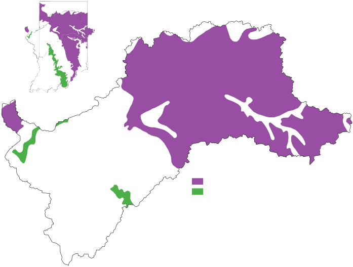
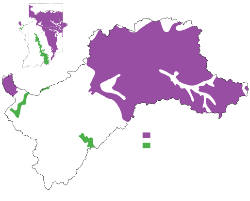
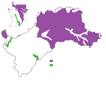
Indiana is underlain by four principal aquifers, the designation the US Geological
Survey (USGS) gives to aquifers that serve as primary water supply sources in a region.
Three of the four principal aquifers in Indiana are consolidated aquifers, sometimes called
bedrock aquifers.
The two largest are comprised of carbonate
rock, and sandstone and
carbonate rock.
The third, a sandstone aquifer along the Ohio River, makes only minor contact with Indiana.
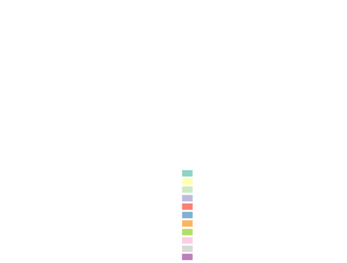
Map showing combined area of North Central Indiana and Wabash Headwaters water
studies by the Indiana Finance Authority and two principal aquifers. The carbonate-rock is
shaded magenta, the sandstone and carbonate rock is shaded green. An inset map in the upper left
shows the study areas in the context of the state of Indiana.
Water availability: baseflow
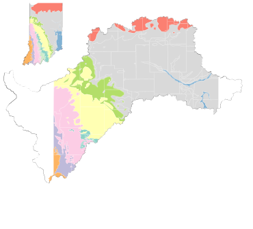
While principal aquifers are the most productive, Indiana is underlain by many aquifers of
varying productivity and depth. Many of the bedrock aquifer systems stretch across wide swaths
of the state.
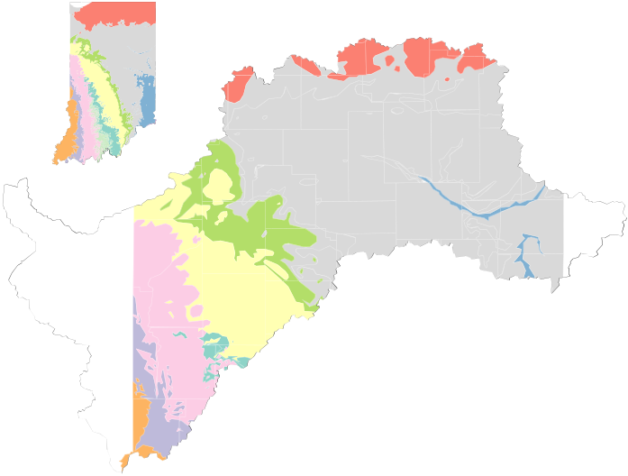
Map showing combined area of North Central Indiana and Wabash Headwaters water
studies by the Indiana Finance Authority and bedrock aquifers within Indiana shaded in different
colors: Blue River, Sanders Groups; Borden Group; Carbondale Group;Coldwater, Ellsworth, Antrim
Shales; Maquoketa Group; McLeansboro Group; New Albany Shale; Raccoon Creek Group; Silurian and
Devonian Carbonates. An inset map in the upper left shows the study area and the aquifers in the
context of the state of Indiana.
Water availability: baseflow
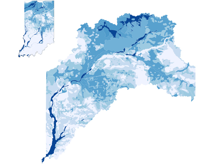
Indiana's unconsolidated aquifers are generally closer to the surface and geologically newer than
their consolidated counterparts.
The state has mapped their yields where data is available. They are a common source
for domestic wells throughout the state and study area.
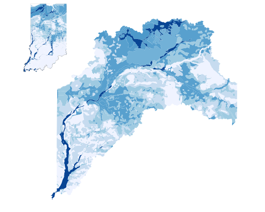
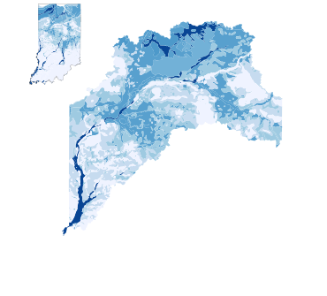
Map showing combined area of North Central Indiana and Wabash Headwaters water
studies by the Indiana Finance Authority as a choropleth with light shades of blue representing
low domestic well range average of 0 gallons per minute capacity transitioning to darker blue
capacity of 50 gallons per minute. An inset map in the upper left shows the study area and the
aquifer capacities in the context of the state of Indiana.
Water availability: baseflow
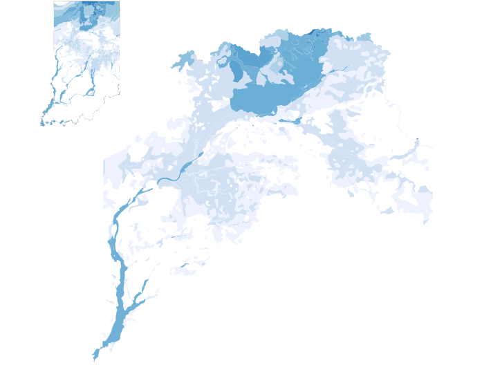
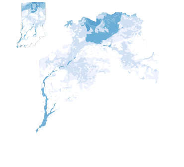
They also support high-capacity withdrawals. Higher yields are found in the northern portions of
the state and study area.
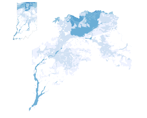
Map showing combined area of North Central Indiana and Wabash Headwaters water
studies by the Indiana Finance Authority as a choropleth with light shades of blue representing
low domestic well range average of 150 gallons per minute capacity transitioning to darker blue
capacity of 1,500 gallons per minute capacity. An inset map in the upper left shows the study
area and the aquifer capacities in the context of the state of Indiana.
Water availability: baseflow
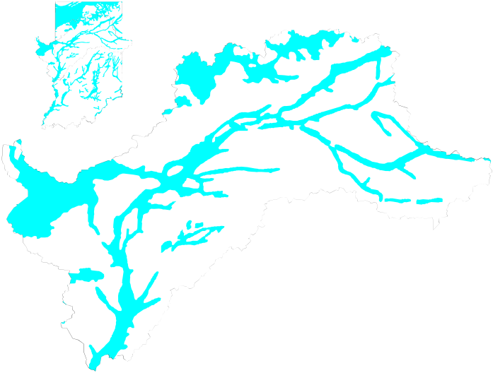
The unconsolidated glacial aquifer system sprawls
across much of the state and beyond. It is the largest water source for public supply and
self-supplied industrial of any principal aquifer, according to the USGS.
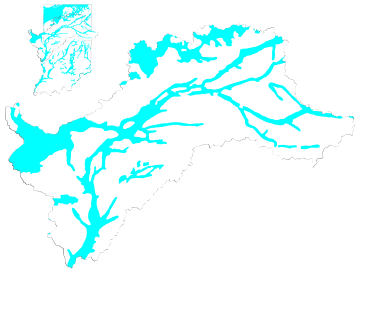
Map showing combined area of North Central Indiana and Wabash Headwaters water
studies by the Indiana Finance Authority and the principal glacial aquifer shaded in teal. An
inset map in the upper left shows the study area and the aquifer in the context of the state of
Indiana.
Water availability: baseflow
Groundwater and surface water interact throughout the hydrologic cycle. Sometimes surface water
is lost to groundwater recharge. At others times, groundwater from aquifers contributes volume
to surface water sources like rivers or streams.
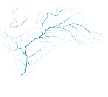
This relationship is not hard to imagine when the state’s rivers and streams are overlaid atop
the glacial aquifer system.
It is through these baseflow contributions, not their total water capacity, that aquifers impact
water availability calculations in these studies.
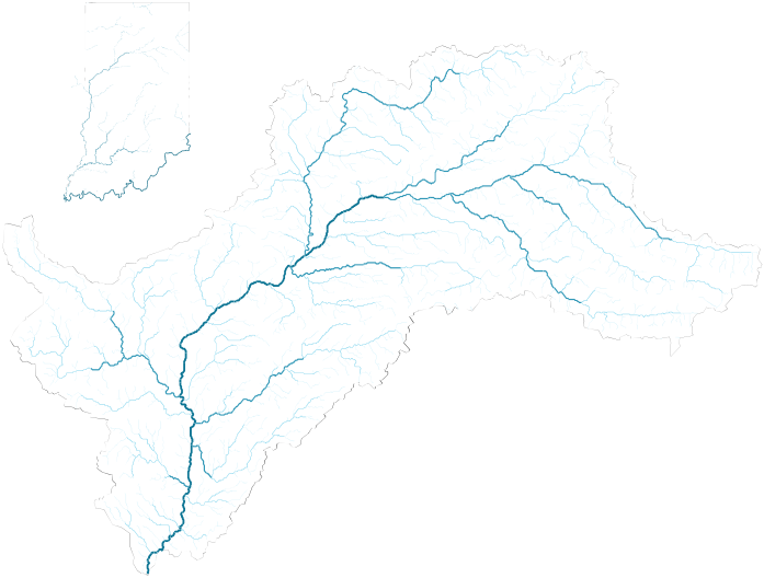
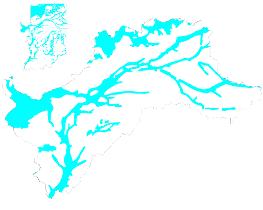
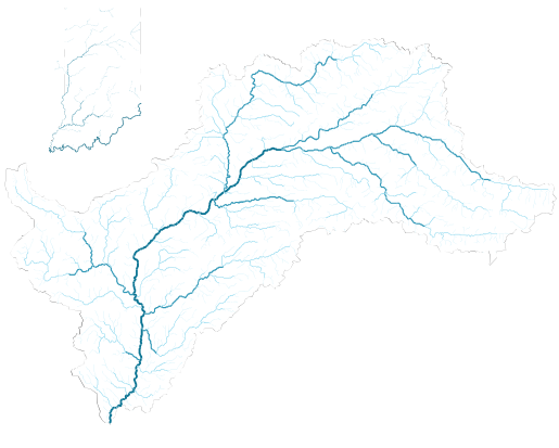
Map showing combined area of North Central Indiana and Wabash Headwaters water
studies by the Indiana Finance Authority and the principal glacial aquifer shaded in teal. Major
and minor waterways are also shown in dark and light blue resepectively. An inset map in the
upper left shows the study area and the aquifer and the waterways in the context of the state of
Indiana.
Water
availability = Net natural
baseflow – net minimum instream flow requirement+subbasin net reservoir
release.
Reservoirs influence water availability by storing or releasing water within a subbasin.
During wet seasons, water that would otherwise be measured at the subbasin outlet is stored
instead, reducing seasonal water availability, sometimes to negative values.
When released, it artificially raises water availability higher than it would otherwise be, a
tactic that can help preserve stream and river flow in dry seasons.
Three reservoirs were identified in each study that influence the seasonality of water
availability in their subbasins and their downstream counterparts.
Set the natural baseflow slider and then
adjust the reservoir operations
slider to see how reservoir storage or release impacts water availability.
Storing water|Releasing water
Illustration of a cylinder with dark blue water and a fixed dashed gray line at
the bottom labeled 'Instream flow requirement.' An indicator and label show Natural baseflow on
the left and a bracked indicator showing Water availability on the right. Both labels move up
and down when users activate the slider control to show relationship between baseflow, the
instream flow requirement and water availability. At high natural baseflow levels, the top of
the cylinder will adjust up to accomodate more water when the Reservoir operations slider moves
toward Releasing water.
Excess water availability
Once the natural baseflow has been calculated, reservoir operations accounted for, and the
minimum instream flow requirements met, excess water availability can be determined
using another formula:
Excess water availability = Water availability– water withdrawals+ return flows.
Water withdrawals occur when groundwater is pumped from aquifers or surface water is drawn from
sources like lakes, rivers or streams.
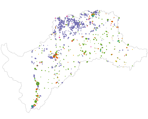
The state of Indiana requires facilities that extract more than 100,000 gallons a day of ground
or surface water to register with the state.
These registered withdrawals are identified by their origin — ground or surface — and categorized
by end-use such as public supply, irrigation, industrial and others.
Aside from energy production, most withdrawals in the study areas come from groundwater.
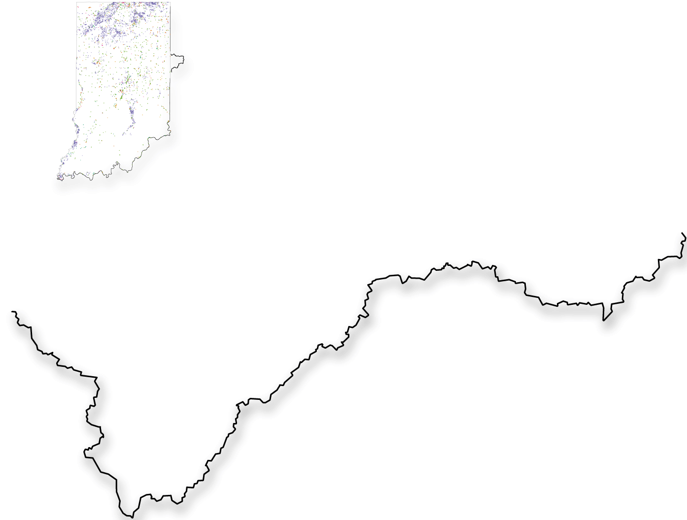
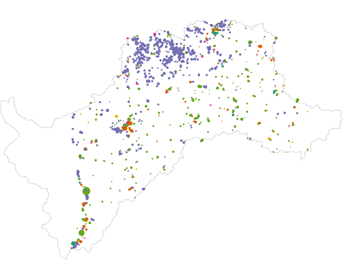
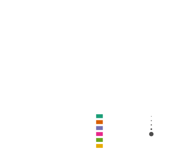
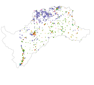
Use the button to visualize how many of Indiana's significant
groundwater withdrawal facilities are found within the principal glacial aquifer boundaries.
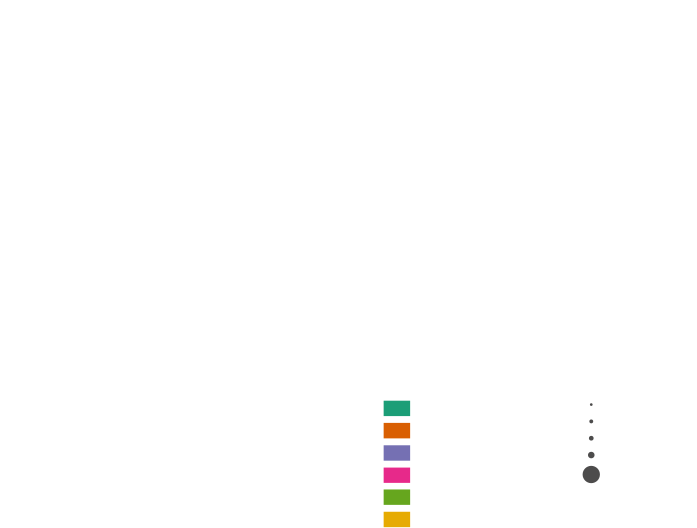
Map showing combined area of North Central Indiana and Wabash Headwaters water
studies by the Indiana Finance Authority and the locations of significant groundwater withdrawal
facilities indicated with circles proportional to the gallons per minute they are capable of
withdrawing ranging from 200 gallons per minute to 13,500. The colors correspond to the end-use
for the withdrawn water. They include energy, industry, irrigation, miscellaneous public supply
and rural use. A button toggles the visibility of the principal glacial aquifer shaded in teal.
An inset map in the upper left shows the study area and withdrawal facilities in the context of
the state of Indiana.
Excess
water
availability = water availability – water withdrawals+return flows.
Water withdrawals vary by amount, season, source, subbasin and intended use but they all reduce
the amount of water available in the subbasin where they occur.
Subbasins with energy production facilities may have high surface water withdrawals from lakes
connected to power plants leading to more consistent year-round demand. In contrast, a subbasin
with high irrigation levels may experience more seasonal withdrawal variability.
Compared to natural baseflow, water withdrawals are a small component of water availability.
Adjust the slider to determine how much water is withdrawn from the
example subbasin. For illustrative purposes their impact is exaggerated.
High withdrawalsLow withdrawals
Illustration of two cylinders with dark blue water. The larger cylinder is
labeled ‘Water within subbasin’ and includes a fixed dashed gray line at the bottom labeled
'Instream flow requirement' a bracketed indicator showing ‘Available water’ on the left. A line
with an arrow connects the larger cylinder to a smaller one in the upper left labeled ‘Water
withdrawals.’ The level in each cylinder changes relative to the Water withdrawals slider
position. Moving the slider to Low withdrawals decreases the blue water level in the small
cylinder and increases it in the larger. Moving the slider to High withdrawals increases the
level in the small cylinder and decreases it in the larger.
Excess
water
availability = water availability – water withdrawals+return
flows.
Water withdrawals can be divided into consumptive and non-consumptive use.
Non-consumptive use returns withdrawn water back to the subbasin.
Water withdrawn for coal-based energy production is considered 99% non-consumptive. Nearly all the water is
returned to the subbasin after use.
Water withdrawn for irrigation, on the other hand, is considered 80% consumptive. Most of the water is lost to
evapotranspiration and does not return to the subbasin.
The percent of consumptive use varies by subbasin and season based on the type of use and other
factors.
Illustration of two cylinders with dark blue water. The larger cylinder is
labeled ‘Water within subbasin’ and includes a fixed dashed gray line at the bottom labeled
'Instream flow requirement' a bracketed indicator showing ‘Available water’ on the left. A line
with an arrow connects the larger cylinder to a smaller one in the upper left labeled ‘Water
withdrawals.’ The upper cylinder has additional water in a light blue shade and a label to the
right indicating the percentage of ‘Non-consumptive use.’ The percentage amount is randomly
generated and updated automatically.
Excess water availability: return flows
The net return flows are the portion of non-consumptive water withdrawals that return to the
subbasin. They can be highly seasonal and can exceed the amount of natural baseflow during very
dry seasons.
Illustration of two cylinders with dark blue water. The larger cylinder is
labeled ‘Water within subbasin’ and includes a fixed dashed gray line at the bottom labeled
'Instream flow requirement' a bracketed indicator showing ‘Available water’ on the left. A line
with an arrow connects the larger cylinder to a smaller one in the upper left labeled ‘Water
withdrawals.’ The upper cylinder has additional water in a light blue shade and a label to the
right indicating the percentage of ‘Non-consumptive use.’ The percentage amount is randomly
generated and updated automatically. A dashed line in the same light blue color as the
non-consumptive use water connects the smaller cylinder in the upper left to the larger cylinder
and is labeled ‘Return flows.’
Excess water availability: return flows
The net returns are added to the available water after the withdrawals are accounted for to
determine excess water availability.
Illustration of two cylinders with dark blue water. The larger cylinder is
labeled ‘Water within subbasin’ and includes a fixed dashed gray line at the bottom labeled
'Instream flow requirement' a bracketed indicator showing ‘Available water’ on the left and
another bracketed indicator labeled ‘Net returns’ that denotes another water level shaded in
light blue directly above the darker blue ‘Available water.’ A bold label that says ‘Excess
water availability’ on the right side of the cylinder with brackets that include entire depth of
both water levels. A line with an arrow connects the larger cylinder to a smaller one in the
upper left labeled ‘Water withdrawals.’ The upper cylinder has additional water in a light blue
shade and a label to the right indicating the percentage of ‘Non-consumptive use.’ The
percentage amount is randomly generated and updated automatically. A dashed line in the same
light blue color as the non-consumptive use water connects the smaller cylinder in the upper
left to the larger cylinder and is labeled ‘Return flows.’
Cumulative excess water availability
Half of the 26 subbasins in the combined study area receive contributions from at least one
upstream subbasin.
These contributions are what distinguish cumulative excess water availability. It
utilizes cumulative versions of the variables used to calculate excess water availability by
incorporating contributions from upstream basins when applicable.
The cumulative excess water availability of the furthest downstream basin in each study area
represents that region's cumulative excess water availability.
For the Wabash Headwaters that is subbasin 10; for the North Central Indiana study, and the
combined study area, that is subbasin 16.
Map showing combined area of North Central Indiana, shaded dark blue, and Wabash
Headwaters, shaded light blue, water studies by the Indiana Finance. The opacity of subbasins
that do not have contributing upstream subbasins is reduced to de-emphasize them. Wabash
Headwaters subbasin 10 and North Central Indiana subbasin 16 are labelled because they represent
the place where the cumulative excess water availability for their collective region is
determined. An inset map in the upper left shows the study area in the context of the state of
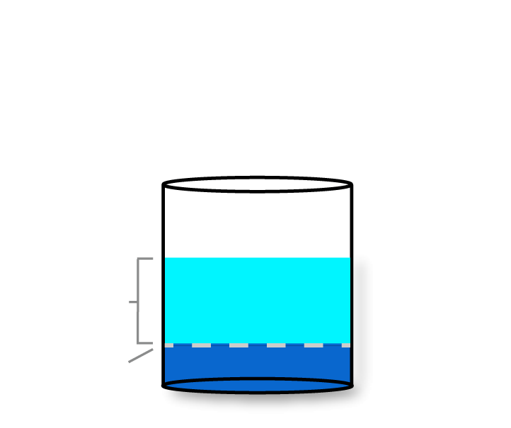
Indiana.
Cumulative excess water availability
Without upstream contributions, a subbasin's cumulative excess water availability is
equal to its excess water availability.
Illustration of a cylinder labeled ‘Subbasin’ with two sections: dark blue water
and lighter blue water. The cylinder has a dashed gray line near the bottom labeled ‘Instream
flow requirement’ that marks the division between the dark and light blue waters. There are two
brackets of identical size on the left and right of the cylinder labeled ‘Excess water
availability’ on the left side and ‘Cumulative excess water availability’ on the right side.
Cumulative excess water availability
A subbasin that receives water from an upstream subbasin adds that excess water availability to
its own to determine its cumulative excess water availability.
Illustration of a cylinder labeled ‘Subbasin’ with two sections: dark blue water
and lighter blue water. The cylinder has a dashed gray line near the bottom labeled ‘Instream
flow requirement’ that marks the division between the dark and light blue waters. A smaller,
similar cylinder appears in the upper left labeled ‘Upstream subbasin’ with an ‘Excess water
availability’ label at the top of its light blue water level. A light blue dashed line connects
the two cylinders with an arrow pointing to the ‘Subbasin’ cylinder. The light blue water level
in the ‘Subbasin’ cylinder rises above the ‘Excess water availability’ bracket, and a second,
larger bracket labeled ‘Cumulative excess water availability’ spans the added height.
Cumulative excess water availability
A subbasin with many upstream contributions will generally have higher cumulative excess water
availability than a subbasin with fewer upstream contributions.
Illustration of a cylinder labeled ‘Subbasin’ with two sections: dark blue water
and lighter blue water. The cylinder has a dashed gray line near the bottom labeled ‘Instream
flow requirement’ that marks the division between the dark and light blue waters. There are two
brackets on the left and right of the cylinder labeled ‘Excess water
availability’ on the left side and ‘Cumulative excess water availability’ on the right side. A
smaller, similar cylinder is in the upper left labeled ‘Upstream subbasin’ with an ‘Excess water
availability’ label on the right side at the top of the light blue water level. A trio of smaller similarly constructed cylinders is in the upper right. Light blue
dashed lines connect the accessory cylinders with an arrow pointing to the primary ‘Subbasin’ cylinder. The light blue
water level in the 'Subbasin' cylinder now exceeds the 'Excess water availability' level that is
not denoted at its top with an additional dashed line across the cylinder. The bracket for the
'Cumulative excess water availability' has adjusted to match the changed level of the light blue
water line.
Cumulative excess water availability
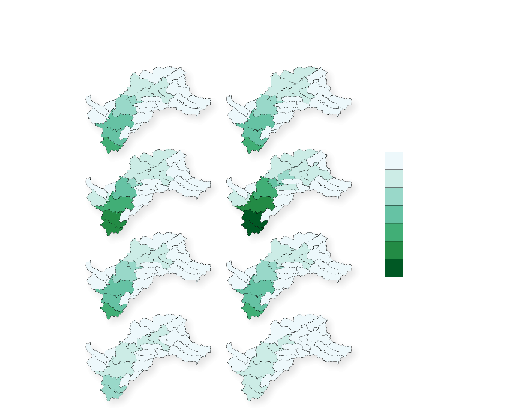
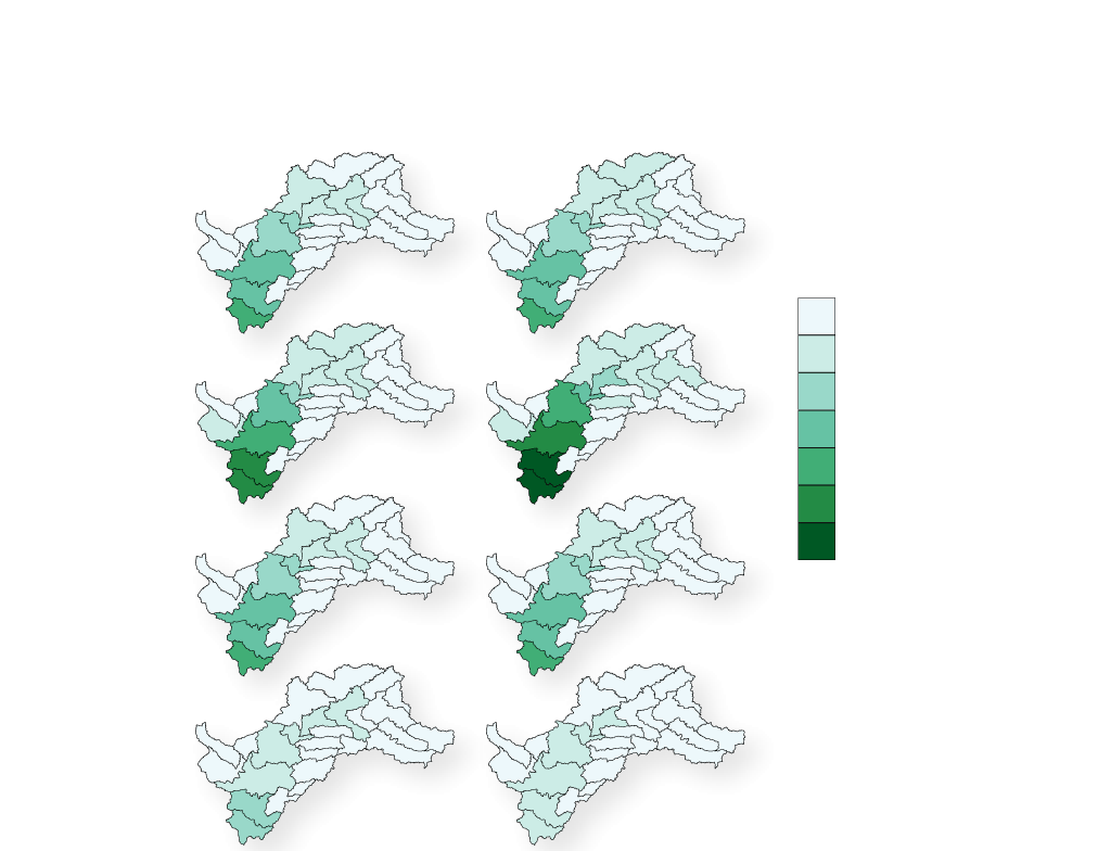
The impacts of upstream contributions on downstream subbasins, and seasonal variation, are
evident in the studies' estimates of historic and future cumulative water availability by season
and subbasin.
The historic period averages seasonal data from 2007 to 2022 while the future projection reflects
estimates for the 2060s.
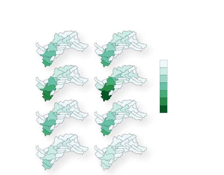
Faceted choropleth map showing combined area of North Central Indiana and Wabash
Headwaters water studies by the Indiana Finance Authority with their subbasins defined by dark
lines and shaded in a range of green colors to indicate cumulative excess water availability in
millions of gallons daily. The range is 12-498 on the low end and 7,727 – 9,964 on the highest
end. The facet is made of two columns - Historic and Future, and four rows – Winter, Spring,
Summer, Fall. The furthest downstream subbasins show the highest totals across the seasons with
Future Spring showing the highest totals.
Cumulative excess water availability
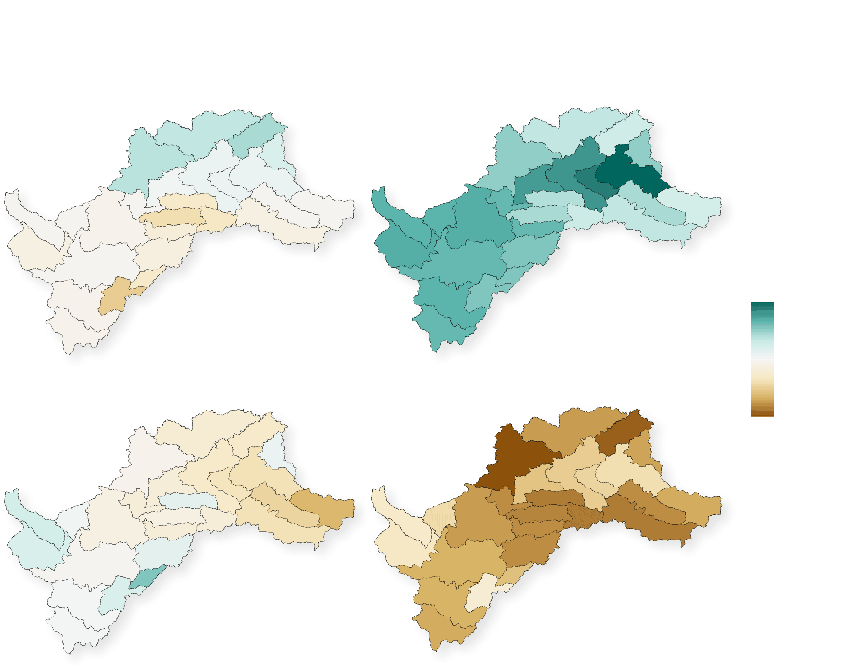
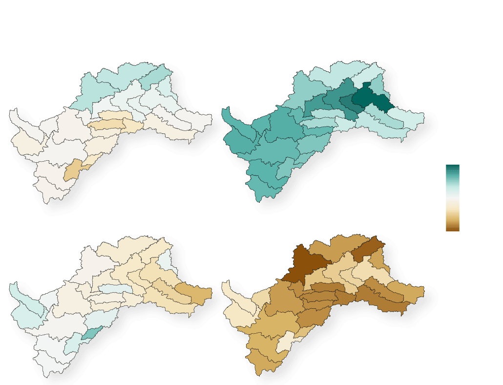
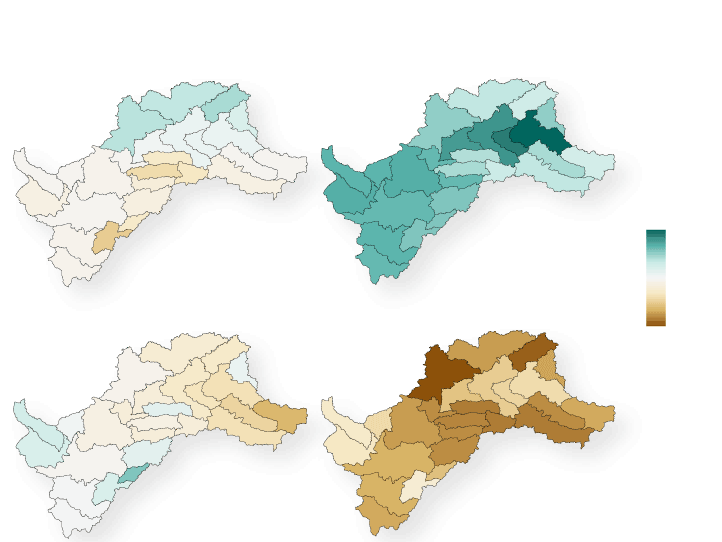
On average, the studies' authors expect wetter springs and drier falls to contribute to
region-wide reductions and surpluses relative to historic conditions in the spring and fall.
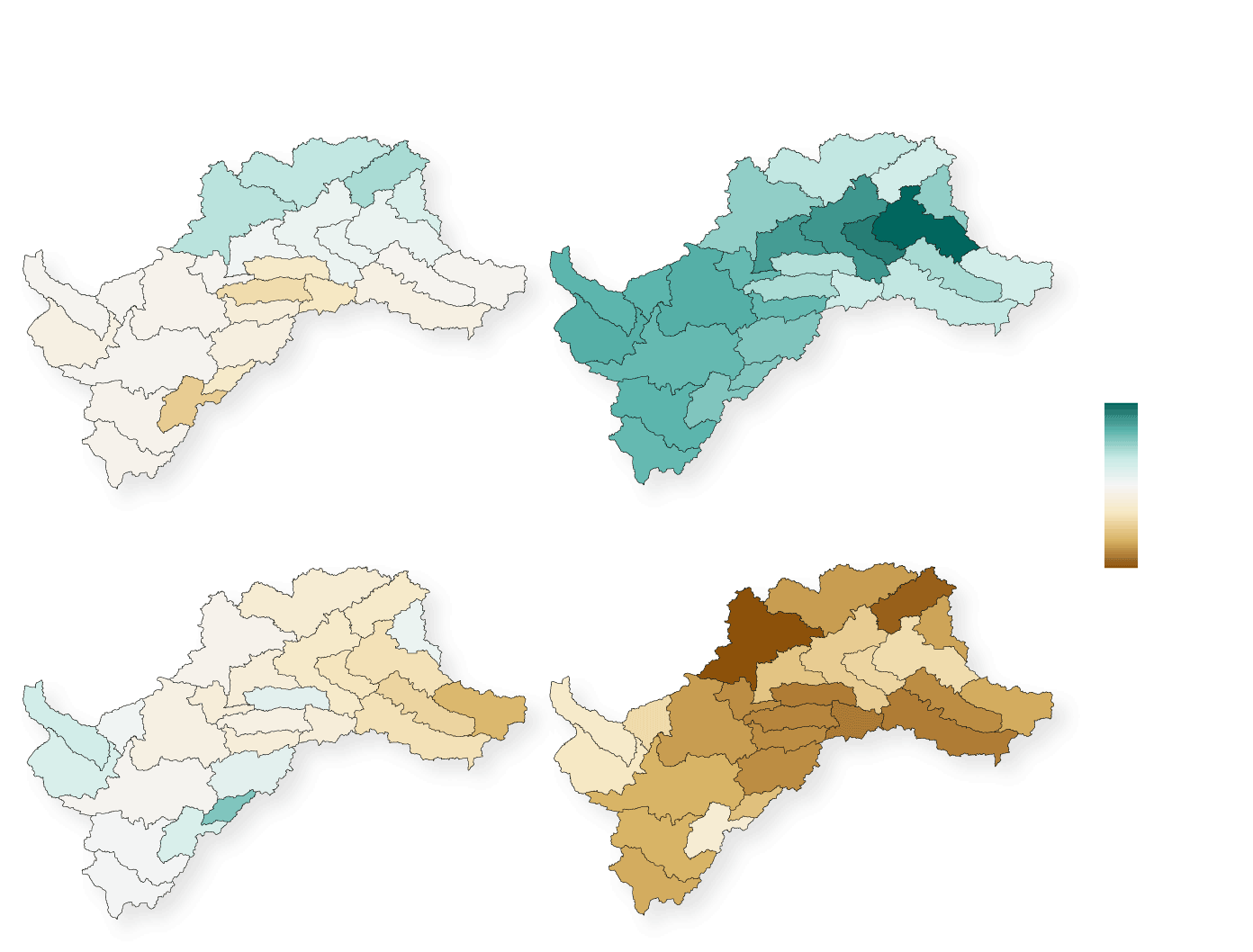
Diverging color faceted choropleth map showing combined area of North Central
Indiana and Wabash Headwaters water studies by the Indiana Finance Authority with their
subbasins defined by dark lines and shaded in a range of brown to blue-green colors to indicate
the percent change in cumulative excess water availability across the four seasons between
historic conditions and projected future conditions. The lightest colors, including white in the
middle of the scale, indicate little to no change. Darker colors indicate higher change. Brown
colors indicate negative change while blue-green colors indicate positive change.
Cumulative excess water availability
Not every year is average, though.
An exceedance curve visualizes how often a certain value is exceeded within a time
frame. They are useful for understanding how extremely wet or dry conditions impact water
availability metrics.
In North Central Indiana subbasin six, spring has the highest cumulative
excess water availability.
In the future, the study projects cumulative excess water availability of about 6,000 million
gallons daily under the wettest conditions, those exceeded six percent of the time. Average
conditions, exceeded about half the time, would be 3,600 million gallons. The driest conditions,
exceeded 94% of the time, would see about 1,200 million gallons daily.
Both summer and winter experience negative water availability during
the driest conditions in the subbasin.
Line chart showing Future cumulative excess water availability exceedances for
North Central Indiana Regional Water Study subbasin 6. Four colored lines correspond to four
seasons: spring-blue, summer-brown, fall-orange, winter-light blue. The y axis is millions of
gallons daily and ranges from 0 to 6,000. The x axis shows exceedance percentage of 0 to 100
from left to right. Three points with labels mark the two extremes and the middle of the Spring
line: “Extremely wet: 6%”, “Average conditions: 53%”, “Extremely dry: 94%.”
Cumulative excess water availability
The cumulative excess water availability values can also be visualized by their area at their
highest, lowest and average exceedance values and color coded to represent conditions:
extremely wet
average
extremely dry
Line chart showing Future cumulative excess water availability exceedances for
North Central Indiana Regional Water Study subbasin 6. Four labeled lines correspond to four
seasons: spring, summer, fall and winter; the spring line is blue, the others shades of gray.
The y axis is millions of gallons daily and ranges from 0 to 6,000. The x axis shows exceedance
percentage of 0 to 100 from left to right. Three points with labels mark the two extremes and
the middle of the Spring line: “Extremely wet: 6%”, “Average conditions: 53%”, “Extremely dry:
94%.” The points are connected via lines with arrows at each end to shaded squares arranged in
vertically on the right side of the chart representing the area of value on the y axis and color
coded. Light peach is extremely wet, orange is average and red is extremely dry.
Cumulative excess water availability
These can be consolidated into a single element for easier comparisons across a season's possible
climate conditions and...
extremely wet
average
extremely dry
Line chart showing Future cumulative excess water availability exceedances for
North Central Indiana Regional Water Study subbasin 6. Four labeled lines correspond to four
seasons: spring, summer, fall and winter; the spring line is blue, the others shades of gray.
The y axis is millions of gallons daily and ranges from 0 to 6,000. The x axis shows exceedance
percentage of 0 to 100 from left to right. Three points with labels mark the two extremes and
the middle of the Spring line: “Extremely wet: 6%”, “Average conditions: 53%”, “Extremely dry:
94%.” The points are connected via lines with arrows at each end to shaded squares on the right
side of the chart representing the area of value on the y axis and color coded. Light peach is
extremely wet, orange is average and red is extremely dry. The three squares overlap each other
in the upper right corner of the chart.
Cumulative excess water availability
...to make it easy to compare the impact of different climate conditions across the four seasons.
The occasional negative water availability that occurs in some subbasins during summer, fall and
winter is visualized as an empty, white square.
extremely wet
average
extremely dry
Line chart showing Future cumulative excess water availability exceedances for
North Central Indiana Regional Water Study subbasin 6. Four labeled lines correspond to four
seasons: spring, summer, fall and winter. The y axis is millions of gallons daily and ranges
from 0 to 6,000. The x axis shows exceedance percentage of 0 to 100 from left to right. Three
points with labels mark the two extremes and the middle of the Spring line: “Extremely wet: 6%”,
“Average conditions: 53%”, “Extremely dry: 94%.” There is a 2 by 2 grid of boxes, each made of
three boxes stacked atop each other that represent the high, low and average exceedance values
for each season. Light peach is extremely wet, orange is average and red is extremely dry. A
label identifies the white squares that indicate negative cumulative excess water availability.
Cumulative excess water availability
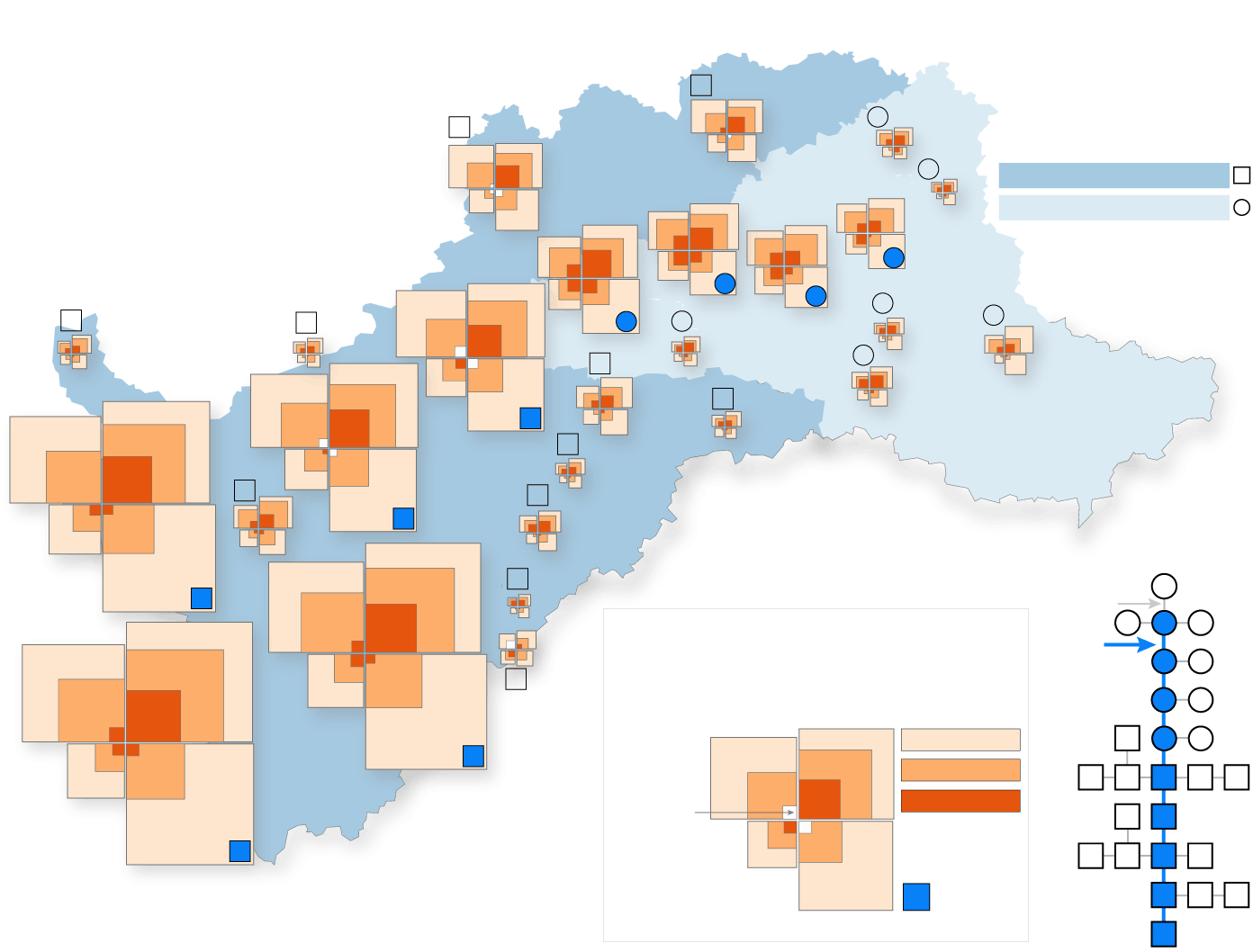
Upstream contributions, especially in subbasins through which the Wabash River flows, magnify the
amount of cumulative excess water availability, especially compared to subbasins with few or no
upstream contributions.
But even those subbasins aren’t immune from the reductions that accompany extremely dry
conditions in the winter, summer and fall.
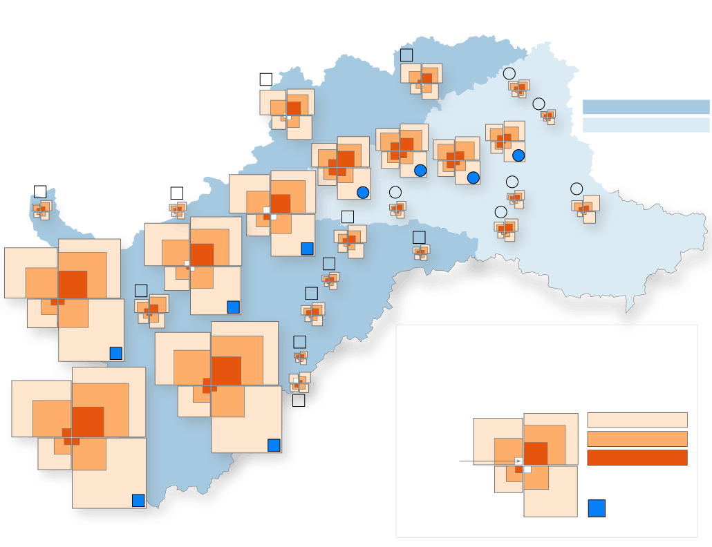
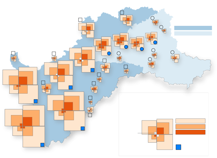
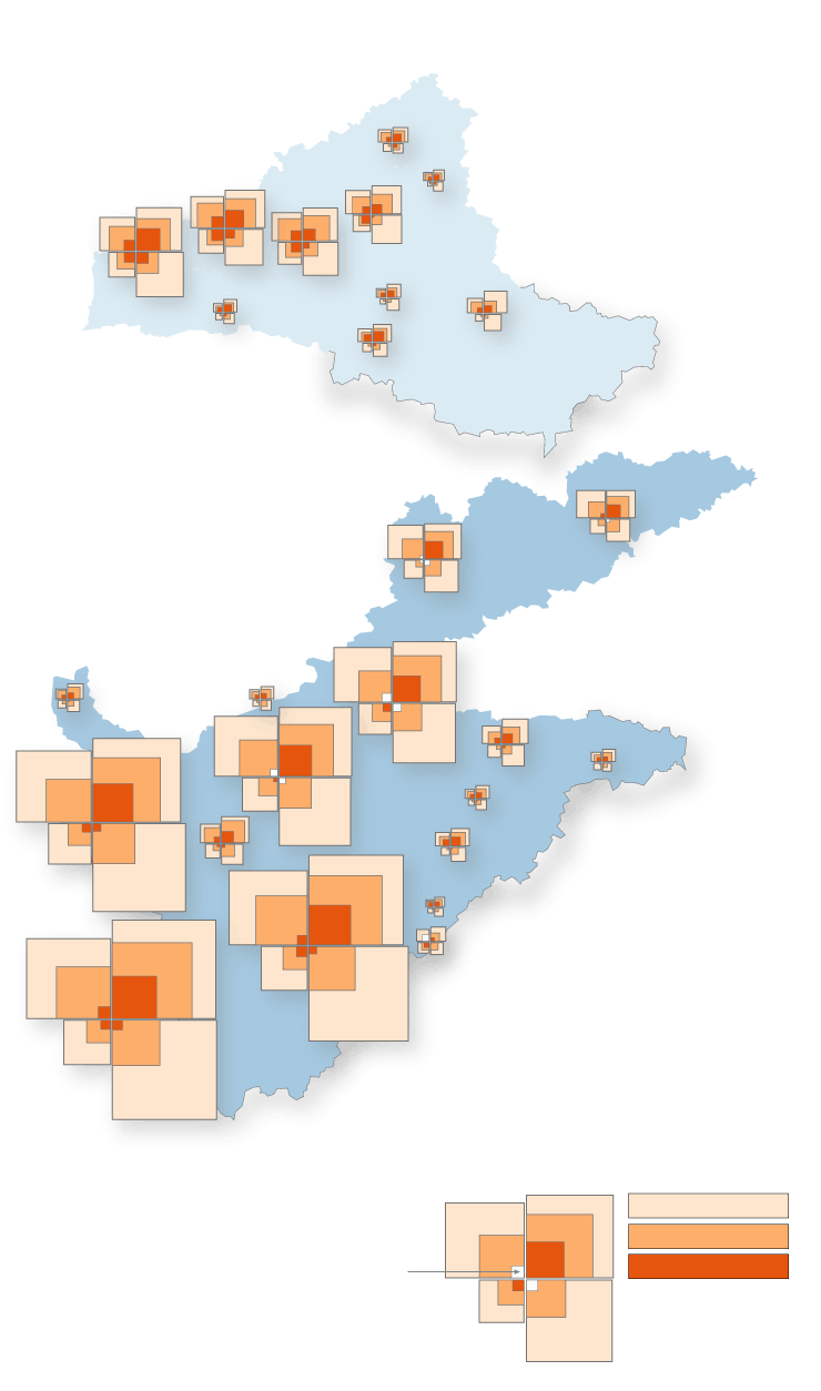
*Location of NCI subbasins 11 and 12 charts are shifted to accomodate chart placement.
Map titled ‘Future cumulative excess water availability by season, subbasin and
climate conditions’ showing combined area of North Central Indiana, shaded dark blue, and Wabash
Headwaters, shaded light blue, water studies by the Indiana Finance Authority. For each
subbasin, four stack’s of three squares each are arranged in a grid representing clockwise from
top left winter, spring, summer and fall. Each season has three boxes stacked within each other,
the color of which denotes the volume of cumulative excess water availability under either
extremely wet (peach color), average (orange color), or extremely dry (red color) conditions.
Each of the subbasin grids includes a shape denoting the water study: a square for the North
Central Indiana study and a circle for the Wabash Headwaters study. The shapes are arranged in a
key labeled ‘Downstream basin flow’ in the lower right to show which subbasins have upstream
contributions and which, shaded dark blue, represent the main stem of the Wabash River.
Recomendations
A few themes emerged from the studies’ detailed recommendations:
Decrease demand:
Implement water loss prevention programs and infrastructure improvements and updates
Promote conservation through public campaigns, incentives and regulations
Increase supply:
Consider conjunctive water use that incorporates both surface and groundwater to meet
demands
Exploration and development of groundwater sources
Reassess reservoir storage and allocation; explore non-reservoir storage potential
Improve data:
Increase data monitoring, collection and sharing for water quality and quantity
Refine analysis methods
*Location of NCI subbasins 11 and 12 charts are shifted to accomodate chart placement.